Backpropogating an LSTM: A Numerical Example

Let’s do this…

We all know LSTM’s are super powerful; So, we should know how they work and how to use them.

Syntactic notes

• Above $\bigodot$ is the element-wise product or Hadamard product.
• Inner products will be represented as $\cdot$
• Outer products will be respresented as $\bigotimes$
• $\sigma$ represents the sigmoid function: $\sigma(x) = \dfrac{1}{1 + e^{-x}}$

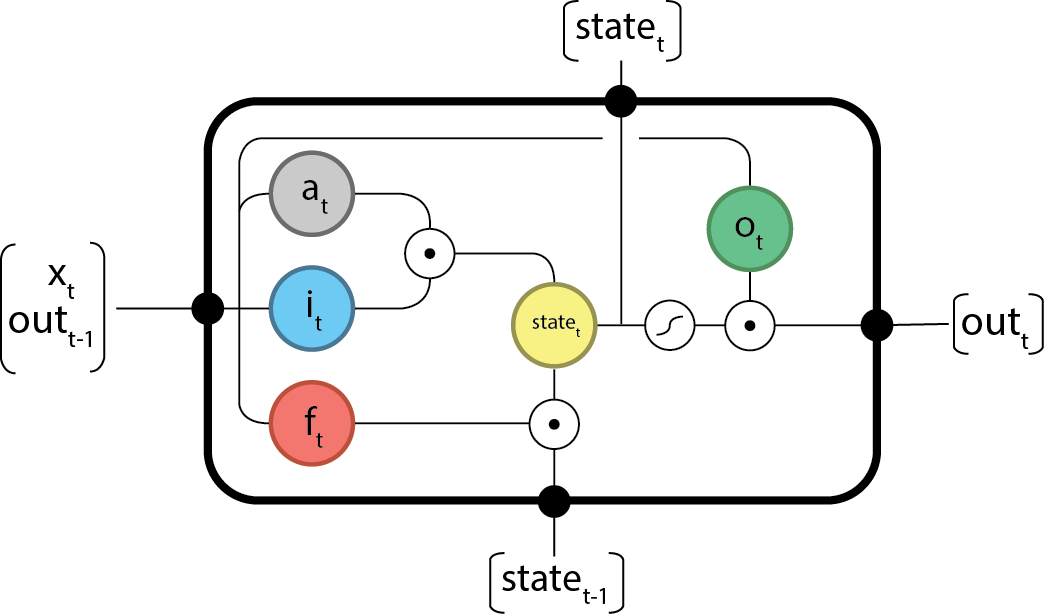
The forward components

The gates are defined as:

• Input activation:
  • $$a_{t} = \tanh(W_{a} \cdot x_{t} + U_{a} \cdot out_{t-1} + b_{a})$$
• Input gate:
  • $$i_{t} = \sigma(W_{i} \cdot x_{t} + U_{i} \cdot out_{t-1} + b_{i})$$
• Forget gate:
  • $$f_{t} = \sigma(W_{f} \cdot x_{t} + U_{f} \cdot out_{t-1} + b_{f})$$
• Output gate:
  • $$o_{t} = \sigma(W_{o} \cdot x_{t} + U_{o} \cdot out_{t-1} + b_{o})$$

Note for simplicity we define:

$$gates_{t} = \begin{bmatrix} a_{t}\\ i_{t}\\ f_{t}\\ o_{t}] \end{bmatrix},\ W = \begin{bmatrix} W_{a}\\ W_{i}\\ W_{f}\\ W_{o} \end{bmatrix},\ U = \begin{bmatrix} U_{a}\\ U_{i}\\ U_{f}\\ U_{o} \end{bmatrix},\ b = \begin{bmatrix} b_{a}\\ b_{i}\\ b_{f}\\ b_{o} \end{bmatrix}$$

Which leads to:

• Internal state:
  • $$state_{t} = a_{t} \odot i_{t} + f_{t} \odot state_{t-1}$$
• Output:
  • $$out_{t} = \tanh(state_{t}) \odot o_{t}$$

The backward components

Given:

• $\Delta_{t}$ the output difference as computed by any subsequent layers (i.e. the rest of your network), and;
• $\Delta out_{t}$ the output difference as computed by the next time-step LSTM (the equation for t-1 is below).

Find:

$$\begin{aligned} \delta out_{t} &= \Delta_{t} + \Delta out_{t}\\ \delta state_{t} &= \delta out_{t} \odot o_{t} \odot (1 - \tanh^{2}(state_{t})) + \delta state_{t+1} \odot f_{t+1}\\ \delta a_{t} &= \delta state_{t} \odot i_{t} \odot (1 - a_{t}^{2})\\ \delta i_{t} &= \delta state_{t} \odot a_{t} \odot i_{t} \odot (1 - i_{t})\\ \delta f_{t} &= \delta state_{t} \odot state_{t-1} \odot f_{t} \odot (1 - f_{t})\\ \delta o_{t} &= \delta out_{t} \odot \tanh(state_{t}) \odot o_{t} \odot (1 - o_{t})\\ \delta x_{t} &= W^{T} \cdot \delta gates_{t}\\ \Delta out_{t-1} &= U^{T} \cdot \delta gates_{t} \end{aligned}$$

The final updates to the internal parameters is computed as:

$$\begin{aligned} \delta W &= \sum\limits^{T}_{t=0} \delta gates_{t} \otimes x_{t}\\ \delta U &= \sum\limits^{T-1}_{t=0} \delta gates_{t+1} \otimes out_{t}\\ \delta b &= \sum\limits^{T}_{t=0} \delta gates_{t+1} \end{aligned}$$

Putting this all together we can begin…

The Example

Let us begin by defining out internal weights:

$$\begin{aligned} W_{a} &= \begin{bmatrix} 0.45\\ 0.25 \end{bmatrix}, U_{a} = \begin{bmatrix} 0.15 \end{bmatrix}, b_{a} = \begin{bmatrix} 0.2 \end{bmatrix}\\ W_{i} &= \begin{bmatrix} 0.95\\ 0.8 \end{bmatrix}, U_{i} = \begin{bmatrix} 0.8 \end{bmatrix}, b_{i} = \begin{bmatrix} 0.65 \end{bmatrix}\\ W_{f} &= \begin{bmatrix} 0.7\\ 0.45 \end{bmatrix}, U_{f} = \begin{bmatrix} 0.1 \end{bmatrix}, b_{f} = \begin{bmatrix} 0.15 \end{bmatrix}\\ W_{o} &= \begin{bmatrix} 0.6\\ 0.4 \end{bmatrix}, U_{o} = \begin{bmatrix} 0.25 \end{bmatrix}, b_{o} = \begin{bmatrix} 0.1 \end{bmatrix} \end{aligned}$$

And now input data:

$$\begin{aligned} x_{0} &= \begin{bmatrix} 1\\ 2 \end{bmatrix} \text{ with label: } 0.5\\ x_{1} &= \begin{bmatrix} 0.5\\ 3 \end{bmatrix} \text{ with label: } 1.25\\ \end{aligned}$$

I’m using a sequence length of two here to demonstrate the unrolling over time of RNNs

Forward @ $t=0$

$$\begin{aligned} &a_{0} = \tanh(W_{a} \cdot x_{0} + U_{a} \cdot out_{-1} + b_{a}) = \tanh(\begin{bmatrix} 0.45\ 0.25 \end{bmatrix} \begin{bmatrix} 1\\ 2 \end{bmatrix} + \begin{bmatrix} 0.15 \end{bmatrix} \begin{bmatrix} 0 \end{bmatrix} + \begin{bmatrix} 0.2 \end{bmatrix}) = 0.81775\\ &i_{0} = \sigma(W_{i} \cdot x_{0} + U_{i} \cdot out_{-1} + b_{i}) = \sigma(\begin{bmatrix} 0.95\ 0.8 \end{bmatrix} \begin{bmatrix} 1\\ 2 \end{bmatrix} + \begin{bmatrix} 0.8 \end{bmatrix} \begin{bmatrix} 0 \end{bmatrix} + \begin{bmatrix} 0.65 \end{bmatrix}) = 0.96083\\ &f_{0} = \sigma(W_{f} \cdot x_{0} + U_{f} \cdot out_{-1} + b_{f}) = \sigma(\begin{bmatrix} 0.7\ 0.45 \end{bmatrix} \begin{bmatrix} 1\\ 2 \end{bmatrix} + \begin{bmatrix} 0.1 \end{bmatrix} \begin{bmatrix} 0 \end{bmatrix} + \begin{bmatrix} 0.15 \end{bmatrix}) = 0.85195\\ &o_{0} = \sigma(W_{o} \cdot x_{0} + U_{o} \cdot out_{-1} + b_{o}) = \sigma(\begin{bmatrix} 0.6\ 0.4 \end{bmatrix} \begin{bmatrix} 1\\ 2 \end{bmatrix} + \begin{bmatrix} 0.25 \end{bmatrix} \begin{bmatrix} 0 \end{bmatrix} + \begin{bmatrix} 0.1 \end{bmatrix}) = 0.81757\\ \\ &state_{0} = a_{0} \odot i_{0} + f_{0} \odot state_{-1} = 0.81775 \times 0.96083 + 0.85195 \times 0 = 0.78572 \\ &out_{0} = \tanh(state_{0}) \odot o_{0} = \tanh(0.78572) \times 0.81757 = 0.53631 \end{aligned}$$

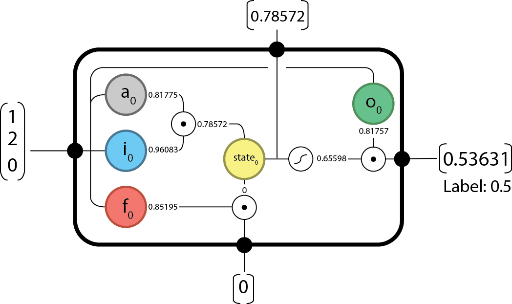
From here, we can pass forward our state and output and begin the next time-step.

Forward @ $t=1$

$$\begin{aligned} &a_{1} = \tanh(W_{a} \cdot x_{1} + U_{a} \cdot out_{0} + b_{a}) = \tanh(\begin{bmatrix} 0.45\ 0.25 \end{bmatrix} \begin{bmatrix} 0.5\\ 3 \end{bmatrix} + \begin{bmatrix} 0.15 \end{bmatrix} \begin{bmatrix} 0.53631 \end{bmatrix} + \begin{bmatrix} 0.2 \end{bmatrix}) = 0.84980\\ &i_{1} = \sigma(W_{i} \cdot x_{1} + U_{i} \cdot out_{0} + b_{i}) = \sigma(\begin{bmatrix} 0.95\ 0.8 \end{bmatrix} \begin{bmatrix} 0.5\\ 3 \end{bmatrix} + \begin{bmatrix} 0.8 \end{bmatrix} \begin{bmatrix} 0.53631 \end{bmatrix} + \begin{bmatrix} 0.65 \end{bmatrix}) = 0.98118\\ &f_{1} = \sigma(W_{f} \cdot x_{1} + U_{f} \cdot out_{0} + b_{f}) = \sigma(\begin{bmatrix} 0.7\ 0.45 \end{bmatrix} \begin{bmatrix} 0.5\\ 3 \end{bmatrix} + \begin{bmatrix} 0.1 \end{bmatrix} \begin{bmatrix} 0.53631 \end{bmatrix} + \begin{bmatrix} 0.15 \end{bmatrix}) = 0.87030\\ &o_{1} = \sigma(W_{o} \cdot x_{1} + U_{o} \cdot out_{0} + b_{o}) = \sigma(\begin{bmatrix} 0.6\ 0.4 \end{bmatrix} \begin{bmatrix} 0.5\\ 3 \end{bmatrix} + \begin{bmatrix} 0.25 \end{bmatrix} \begin{bmatrix} 0.53631 \end{bmatrix} + \begin{bmatrix} 0.1 \end{bmatrix}) = 0.84993\\ \\ &state_{1} = a_{1} \odot i_{1} + f_{1} \odot state_{0} = 0.84980 \times 0.98118 + 0.87030 \times 0.78572 = 1.5176 \\ &out_{1} = \tanh(state_{1}) \odot o_{1} = \tanh(1.5176) \times 0.84993 = 0.77197 \end{aligned}$$

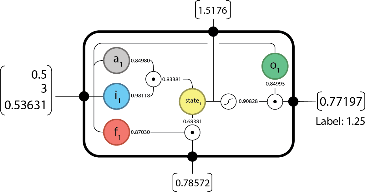
And since we’re done our sequence we have everything we need to begin backpropogating.

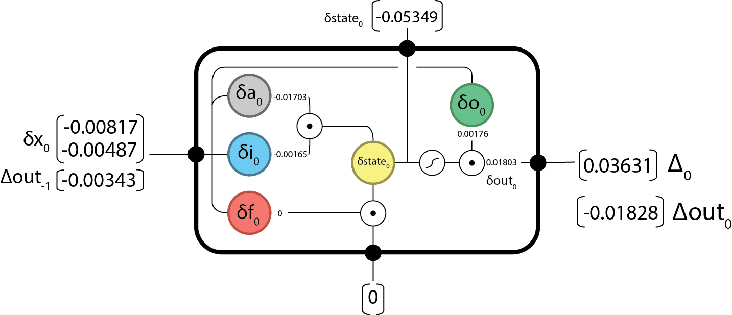
Backward @ $t=1$

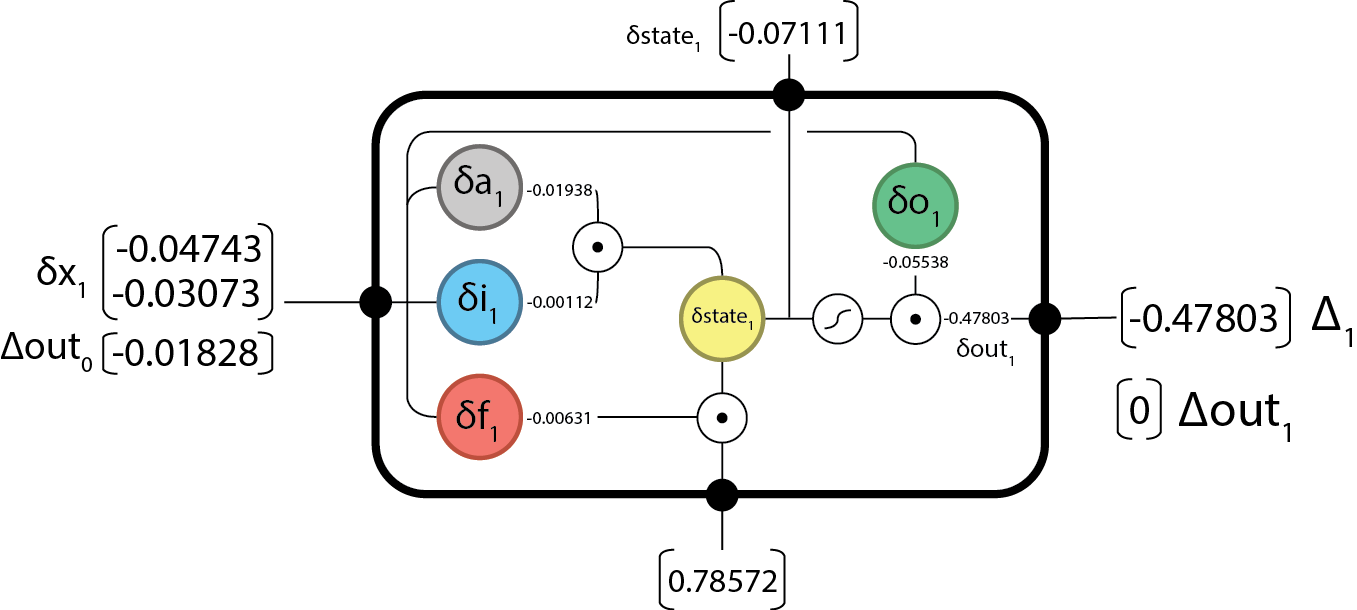
First we’ll need to compute the difference in output from the expected (label).

Note for this we’ll be using L2 Loss: $E(x, \hat x) = \dfrac{(x - \hat x)^{2}}{2}$. The derivate w.r.t. $x$ is $\partial_{x}E(x, \hat x) = x - \hat x$.

$$\begin{aligned} \Delta_{1} = \partial_{x}E = 0.77197 - 1.25 = -0.47803 \end{aligned}$$

$\Delta out_{1} = 0$ because there are no future time-steps.

$$\begin{aligned} \delta out_{1} &= \Delta_{1} + \Delta out_{1} = -0.47803 + 0 = -0.47803\\ \delta state_{1} &= \delta out_{1} \odot o_{1} \odot (1 - \tanh^{2}(state_{1})) + \delta state_{2} \odot f_{2} = -0.47803 \times 0.84993 \times (1 - \tanh^{2}(1.5176)) + 0 \times 0 = -0.07111\\ \delta a_{1} &= \delta state_{1} \odot i_{1} \odot (1 - a_{1}^{2}) = -0.07111 \times 0.98118 \times (1 - 0.84980^{2}) = -0.01938\\ \delta i_{1} &= \delta state_{1} \odot a_{1} \odot i_{1} \odot (1 - i_{1}) = -0.07111 \times 0.84980 \times 0.98118 \times (1 - 0.98118) = -0.00112\\ \delta f_{1} &= \delta state_{1} \odot state_{0} \odot f_{1} \odot (1 - f_{1}) = -0.07111 \times 0.78572 \times 0.87030 \times (1 - 0.87030) = -0.00631\\ \delta o_{1} &= \delta out_{1} \odot \tanh(state_{1}) \odot o_{1} \odot (1 - o_{1}) = -0.47803 \times \tanh(1.5176) \times 0.84993 \times (1 - 0.84993) = -0.05538\\ \\ \delta x_{1} &= W^{T} \cdot \delta gates_{1}\\ &= \begin{bmatrix} 0.45 \ 0.95 \ 0.70 \ 0.60 \\ 0.25 \ 0.80 \ 0.45 \ 0.40\end{bmatrix} \begin{bmatrix} -0.01938 \\ -0.00112 \\ -0.00631 \\ -0.05538\end{bmatrix} = \begin{bmatrix} -0.04743 \\ -0.03073 \end{bmatrix}\\ \Delta out_{0} &= U^{T} \cdot \delta gates_{1}\\ &= \begin{bmatrix} 0.15 \ 0.80 \ 0.10 \ 0.25 \end{bmatrix} \begin{bmatrix} -0.01938 \\ -0.00112 \\ -0.00631 \\ -0.05538\end{bmatrix} = -0.01828\\ \end{aligned}$$

Now we can pass back our $\Delta out_{0}$ and continue on computing…

Backward @ $t=0$

$$\begin{aligned} \Delta_{0} &= \partial_{x}E = 0.53631 - 0.5 = 0.03631\\ \Delta out_{0} &= -0.01828, \text{ passed back from T=1}\\ \\ \delta out_{0} &= \Delta_{0} + \Delta out_{0} = 0.03631 + -0.01828 = 0.01803\\ \delta state_{0} &= \delta out_{0} \odot o_{0} \odot (1 - \tanh^{2}(state_{0})) + \delta state_{1} \odot f_{1} = 0.01803 \times 0.81757 \times (1 - \tanh^{2}(0.78572)) + -0.07111 \times 0.87030 = -0.05349\\ \delta a_{0} &= \delta state_{0} \odot i_{0} \odot (1 - a_{0}^{2}) = -0.05349 \times 0.96083 \times (1 - 0.81775^{2}) = -0.01703\\ \delta i_{0} &= \delta state_{0} \odot a_{0} \odot i_{0} \odot (1 - i_{0}) = -0.05349 \times 0.81775 \times 0.96083 \times (1 - 0.96083) = -0.00165\\ \delta f_{0} &= \delta state_{0} \odot state_{-1} \odot f_{0} \odot (1 - f_{0}) = -0.05349 \times 0 \times 0.85195 \times (1 - 0.85195) = 0\\ \delta o_{0} &= \delta out_{0} \odot \tanh(state_{0}) \odot o_{0} \odot (1 - o_{0}) = 0.01803 \times \tanh(0.78572) \times 0.81757 \times (1 - 0.81757) = 0.00176\\ \\ \delta x_{0} &= W^{T} \cdot \delta gates_{0}\\ &= \begin{bmatrix} 0.45 \ 0.95 \ 0.70 \ 0.60 \\ 0.25 \ 0.80 \ 0.45 \ 0.40\end{bmatrix} \begin{bmatrix} -0.01703 \\ -0.00165 \\ 0 \\ 0.00176 \end{bmatrix} = \begin{bmatrix} -0.00817 \\ -0.00487 \end{bmatrix}\\ \Delta out_{-1} &= U^{T} \cdot \delta gates_{1}\\ &= \begin{bmatrix} 0.15 \ 0.80 \ 0.10 \ 0.25 \end{bmatrix} \begin{bmatrix} -0.01703 \\ -0.00165 \\ 0 \\ 0.00176 \end{bmatrix} = -0.00343\\ \end{aligned}$$

And we’re done the backward step!

Now we’ll need to update our internal parameters according to whatever solving algorithm you’ve chosen. I’m going to use a simple Stochastic Gradient Descent (SGD) update with learning rate: $\lambda = 0.1$.

We’ll need to compute how much our weights are going to change by:

$$\begin{aligned} \delta W &= \sum\limits^{T}_{t=0} \delta gates_{t} \otimes x_{t}\\ &= \begin{bmatrix} -0.01703 \\ -0.00165 \\ 0 \\ 0.00176 \end{bmatrix} \begin{bmatrix} 1.0 \ 2.0 \end{bmatrix} + \begin{bmatrix} -0.01938 \\ -0.00112 \\ -0.00631 \\ -0.05538\end{bmatrix} \begin{bmatrix} 0.5 \ 3.0 \end{bmatrix} = \begin{bmatrix} -0.02672 \ -0.0922 \\ -0.00221 \ -0.00666 \\ -0.00316 \ -0.01893 \\ -0.02593 \ -0.16262 \end{bmatrix}\\ \delta U &= \sum\limits^{T-1}_{t=0} \delta gates_{t+1} \otimes out_{t}\\ &= \begin{bmatrix} -0.01938 \\ -0.00112 \\ -0.00631 \\ -0.05538\end{bmatrix} \begin{bmatrix} 0.53631 \end{bmatrix} = \begin{bmatrix} -0.01039 \\ -0.00060 \\ -0.00338 \\ -0.02970 \end{bmatrix}\\ \delta b &= \sum\limits^{T}_{t=0} \delta gates_{t+1}\\ &= \begin{bmatrix} -0.01703 \\ -0.00165 \\ 0 \\ 0.00176 \end{bmatrix} + \begin{bmatrix} -0.01938 \\ -0.00112 \\ -0.00631 \\ -0.05538\end{bmatrix} = \begin{bmatrix} -0.03641 \\ -0.00277 \\ -0.00631 \\ -0.05362 \end{bmatrix} \end{aligned}$$

And updating out parameters based on the SGD update function: $W^{new} = W^{old} - \lambda * \delta W^{old}$ we get our new weight set:

$$\begin{aligned} W_{a} &= \begin{bmatrix} 0.45267\\ 0.25922 \end{bmatrix}, U_{a} = \begin{bmatrix} 0.15104 \end{bmatrix}, b_{a} = \begin{bmatrix} 0.20364 \end{bmatrix}\\ W_{i} &= \begin{bmatrix} 0.95022\\ 0.80067 \end{bmatrix}, U_{i} = \begin{bmatrix} 0.80006 \end{bmatrix}, b_{i} = \begin{bmatrix} 0.65028 \end{bmatrix}\\ W_{f} &= \begin{bmatrix} 0.70031\\ 0.45189 \end{bmatrix}, U_{f} = \begin{bmatrix} 0.10034 \end{bmatrix}, b_{f} = \begin{bmatrix} 0.15063 \end{bmatrix}\\ W_{o} &= \begin{bmatrix} 0.60259\\ 0.41626 \end{bmatrix}, U_{o} = \begin{bmatrix} 0.25297 \end{bmatrix}, b_{o} = \begin{bmatrix} 0.10536 \end{bmatrix} \end{aligned}$$

And that completes one iteration of solving an LSTM cell!

Of course, this whole process is sequential in nature and a small error will render all subsequent calculations useless, so if you catch ANYTHING email me at hello@aidangomez.ca